Decorator JITs – Python as a DSL

Preface – where we’re going

The goal is to explain how different kinds of jit decorators work by using
a simplified, educational example that implements several approaches from
scratch. All the approaches featured in this post will be using this flow:

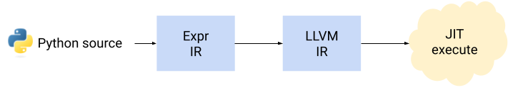
These are the steps that happen when a Python function wrapped with
our educational jit decorator is called:

1. The function is translated to an “expression IR” – Expr.
2. This expression IR is converted to LLVM IR.
3. Finally, the LLVM IR is JIT-executed.

Steps (2) and (3) use llvmlite; I’ve
written about llvmlite before, see this post
and also the pykaleidoscope project.
For an introduction to JIT compilation, be sure to read this
and maybe also the series of posts starting here.

First, let’s look at the Expr IR. Here we’ll make a big simplification –
only supporting functions that define a single expression, e.g.:

def expr2(a, b, c, d):
    return (a + d) * (10 - c) + b + d / c

Naturally, this can be easily generalized – after all, LLVM IR can be used to
express fully general computations.

Here are the Expr data structures:

class Expr:
    pass

@dataclass
class ConstantExpr(Expr):
    value: float

@dataclass
class VarExpr(Expr):
    name: str
    arg_idx: int

class Op(Enum):
    ADD = "+"
    SUB = "-"
    MUL = "*"
    DIV = "/"

@dataclass
class BinOpExpr(Expr):
    left: Expr
    right: Expr
    op: Op

To convert an Expr into LLVM IR and JIT-execute it, we’ll use this function:

def llvm_jit_evaluate(expr: Expr, *args: float) -> float:
    """Use LLVM JIT to evaluate the given expression with *args.

    expr is an instance of Expr. *args are the arguments to the expression, each
    a float. The arguments must match the arguments the expression expects.

    Returns the result of evaluating the expression.
    """
    llvm.initialize()
    llvm.initialize_native_target()
    llvm.initialize_native_asmprinter()
    llvm.initialize_native_asmparser()

    cg = _LLVMCodeGenerator()
    modref = llvm.parse_assembly(str(cg.codegen(expr, len(args))))

    target = llvm.Target.from_default_triple()
    target_machine = target.create_target_machine()
    with llvm.create_mcjit_compiler(modref, target_machine) as ee:
        ee.finalize_object()
        cfptr = ee.get_function_address("func")
        cfunc = CFUNCTYPE(c_double, *([c_double] * len(args)))(cfptr)
        return cfunc(*args)

It uses the _LLVMCodeGenerator class to actually generate LLVM IR from Expr.
This process is straightforward and covered extensively in the resources I
linked to earlier; take a look at the full code here.

My goal with this architecture is to make things simple, but not too simple.
On one hand – there are several simplifications: only single expressions are
supported, very limited set of operators, etc. It’s very easy to extend this!
On the other hand, we could have just trivially evaluated the Expr
without resorting to LLVM IR; I do want to show a more complete compilation
pipeline, though, to demonstrate that an arbitrary amount of complexity can
be hidden behind these simple interfaces.

With these building blocks in hand, we can review the strategies used by
jit decorators to convert Python functions into Exprs.

AST-based JIT

Python comes with powerful code reflection and introspection capabilities out
of the box. Here’s the astjit decorator:

def astjit(func):
    @functools.wraps(func)
    def wrapper(*args, **kwargs):
        if kwargs:
            raise ASTJITError("Keyword arguments are not supported")
        source = inspect.getsource(func)
        tree = ast.parse(source)

        emitter = _ExprCodeEmitter()
        emitter.visit(tree)
        return llvm_jit_evaluate(emitter.return_expr, *args)

    return wrapper

This is a standard Python decorator. It takes a function and returns another
function that will be used in its place (functools.wraps ensures that
function attributes like the name and docstring of the wrapper match the
wrapped function).

Here’s how it’s used:

from astjit import astjit

@astjit
def some_expr(a, b, c):
    return b / (a + 2) - c * (b - a)

print(some_expr(2, 16, 3))

After astjit is applied to some_expr, what some_expr holds is the
wrapper. When some_expr(2, 16, 3) is called, the wrapper is invoked with
*args = [2, 16, 3].

The wrapper obtains the AST of the wrapped function, and then uses
_ExprCodeEmitter to convert this AST into an Expr:

class _ExprCodeEmitter(ast.NodeVisitor):
    def __init__(self):
        self.args = []
        self.return_expr = None
        self.op_map = 
            ast.Add: Op.ADD,
            ast.Sub: Op.SUB,
            ast.Mult: Op.MUL,
            ast.Div: Op.DIV,
        

    def visit_FunctionDef(self, node):
        self.args = [arg.arg for arg in node.args.args]
        if len(node.body) != 1 or not isinstance(node.body[0], ast.Return):
            raise ASTJITError("Function must consist of a single return statement")
        self.visit(node.body[0])

    def visit_Return(self, node):
        self.return_expr = self.visit(node.value)

    def visit_Name(self, node):
        try:
            idx = self.args.index(node.id)
        except ValueError:
            raise ASTJITError(f"Unknown variable node.id")
        return VarExpr(node.id, idx)

    def visit_Constant(self, node):
        return ConstantExpr(node.value)

    def visit_BinOp(self, node):
        left = self.visit(node.left)
        right = self.visit(node.right)
        try:
            op = self.op_map[type(node.op)]
            return BinOpExpr(left, right, op)
        except KeyError:
            raise ASTJITError(f"Unsupported operator node.op")

When _ExprCodeEmitter finishes visiting the AST it’s given, its
return_expr field will contain the Expr representing the function’s
return value. The wrapper then invokes llvm_jit_evaluate with this Expr.

Note how our decorator interjects into the regular Python execution process.
When some_expr is called, instead of the standard Python compilation and
execution process (code is compiled into bytecode, which is then executed
by the VM), we translate its code to our own representation and emit LLVM from
it, and then JIT execute the LLVM IR. While it seems kinda pointless in this
artificial example, in reality this means we can execute the function’s code
in any way we like.

Bytecode-based JIT

Python is a fairly complicated language with a lot of features. Therefore,
if our JIT has to support some large portion of Python semantics, it may make
sense to leverage more of Python’s own compiler. Concretely, we can have it
compile the wrapped function all the way to bytecode,
and start our translation from there.

Here’s the bytecodejit decorator that does just this :

def bytecodejit(func):
    @functools.wraps(func)
    def wrapper(*args, **kwargs):
        if kwargs:
            raise BytecodeJITError("Keyword arguments are not supported")

        expr = _emit_exprcode(func)
        return llvm_jit_evaluate(expr, *args)

    return wrapper


def _emit_exprcode(func):
    bc = func.__code__
    stack = []
    for inst in dis.get_instructions(func):
        match inst.opname:
            case "LOAD_FAST":
                idx = inst.arg
                stack.append(VarExpr(bc.co_varnames[idx], idx))
            case "LOAD_CONST":
                stack.append(ConstantExpr(inst.argval))
            case "BINARY_OP":
                right = stack.pop()
                left = stack.pop()
                match inst.argrepr:
                    case "+":
                        stack.append(BinOpExpr(left, right, Op.ADD))
                    case "-":
                        stack.append(BinOpExpr(left, right, Op.SUB))
                    case "*":
                        stack.append(BinOpExpr(left, right, Op.MUL))
                    case "/":
                        stack.append(BinOpExpr(left, right, Op.DIV))
                    case _:
                        raise BytecodeJITError(f"Unsupported operator inst.argval")
            case "RETURN_VALUE":
                if len(stack) != 1:
                    raise BytecodeJITError("Invalid stack state")
                return stack.pop()
            case "RESUME" | "CACHE":
                # Skip nops
                pass
            case _:
                raise BytecodeJITError(f"Unsupported opcode inst.opname")

The Python VM is a stack machine; so we emulate a stack to convert the
function’s bytecode to Expr IR (a bit like an RPN evaluator).
As before, we then use our llvm_jit_evaluate utility function to lower
Expr to LLVM IR and JIT execute it.

Using this JIT is as simple as the previous one – just swap astjit
for bytecodejit:

from bytecodejit import bytecodejit

@bytecodejit
def some_expr(a, b, c):
    return b / (a + 2) - c * (b - a)

print(some_expr(2, 16, 3))

Tracing-based JIT

The two approaches we’ve seen so far are similar in many ways – both rely on
Python’s introspection capabilities to compile the source code of the JIT-ed
function to some extent (one to AST, the other all the way to bytecode), and
then work on this lowered representation.

The tracing strategy is very different. It doesn’t analyze the source code of
the wrapped function at all – instead, it traces its execution by means of
specially-boxed arguments, leveraging overloaded operators and functions, and
then works on the generated trace.

The code implementing this for our smile demo is surprisingly compact:

def tracejit(func):
    @functools.wraps(func)
    def wrapper(*args, **kwargs):
        if kwargs:
            raise TraceJITError("Keyword arguments are not supported")

        argspec = inspect.getfullargspec(func)

        argboxes = []
        for i, arg in enumerate(args):
            if i >= len(argspec.args):
                raise TraceJITError("Too many arguments")
            argboxes.append(_Box(VarExpr(argspec.args[i], i)))

        out_box = func(*argboxes)
        return llvm_jit_evaluate(out_box.expr, *args)

    return wrapper

Each runtime argument of the wrapped function is assigned a VarExpr, and
that is placed in a _Box, a placeholder class which lets us
do operator overloading:

@dataclass
class _Box:
    expr: Expr

_Box.__add__ = _Box.__radd__ = _register_binary_op(Op.ADD)
_Box.__sub__ = _register_binary_op(Op.SUB)
_Box.__rsub__ = _register_binary_op(Op.SUB, reverse=True)
_Box.__mul__ = _Box.__rmul__ = _register_binary_op(Op.MUL)
_Box.__truediv__ = _register_binary_op(Op.DIV)
_Box.__rtruediv__ = _register_binary_op(Op.DIV, reverse=True)

The remaining key function is _register_binary_op:

def _register_binary_op(opcode, reverse=False):
    """Registers a binary opcode for Boxes.

    If reverse is True, the operation is registered as arg2 <op> arg1,
    instead of arg1 <op> arg2.
    """

    def _op(arg1, arg2):
        if reverse:
            arg1, arg2 = arg2, arg1
        box1 = arg1 if isinstance(arg1, _Box) else _Box(ConstantExpr(arg1))
        box2 = arg2 if isinstance(arg2, _Box) else _Box(ConstantExpr(arg2))
        return _Box(BinOpExpr(box1.expr, box2.expr, opcode))

    return _op

To understand how this works, consider this trivial example:

@tracejit
def add(a, b):
    return a + b

print(add(1, 2))

After the decorated function is defined, add holds the wrapper function
defined inside tracejit. When add(1, 2) is called, the wrapper runs:

1. For each argument of add itself (that is a and b), it creates
   a new _Box holding a VarExpr. This denotes a named variable in
   the Expr IR.
2. It then calls the wrapped function, passing it the boxes as runtime
   parameters.
3. When (the wrapped) add runs, it invokes a + b. This is caught by the overloaded
   __add__ operator of _Box, and it creates a new BinOpExpr with
   the VarExprs representing a and b as children. This
   BinOpExpr is then returned .
4. The wrapper unboxes the returned Expr and passes it to
   llvm_jit_evaluate to emit LLVM IR from it and JIT execute it with the
   actual runtime arguments of the call: 1, 2.

This might be a little mind-bending at first, because there are two different
executions that happen:

• The first is calling the wrapped add function itself, letting the Python
  interpreter run it as usual, but with special arguments that build up the IR
  instead of doing any computations. This is the tracing step.
• The second is lowering this IR our tracing step built into LLVM IR and then
  JIT executing it with the actual runtime argument values 1, 2; this is
  the execution step.

This tracing approach has some interesting characteristics. Since we don’t
have to analyze the source of the wrapped functions but only trace through
the execution, we can “magically” support a much richer set of programs, e.g.:

@tracejit
def use_locals(a, b, c):
    x = a + 2
    y = b - a
    z = c * x
    return y / x - z

print(use_locals(2, 8, 11))

This just works with our basic tracejit. Since Python variables are
placeholders (references) for values, our tracing step is oblivious to them – it
follows the flow of values. Another example:

@tracejit
def use_loop(a, b, c):
    result = 0
    for i in range(1, 11):
        result += i
    return result + b * c

print(use_loop(10, 2, 3))

This also just works! The created Expr will be a long chain of BinExpr
additions of i‘s runtime values through the loop, added to the BinExpr
for b * c.

This last example also leads us to a limitation of the tracing approach; the
loop cannot be data-dependent – it cannot depend on the function’s arguments,
because the tracing step has no concept of runtime values and wouldn’t know
how many iterations to run through; or at least, it doesn’t know this unless
we want to perform the tracing run for every runtime execution .

The tracing approach is useful in several domains, most notably
automatic differentiation (AD).
For a slightly deeper taste, check out my radgrad project.

import jax

@jax.jit
def sum_datadep(a, b, count):
    total = a
    for i in range(count):
        total += b
    return total

print(sum_datadep(10, 3, 3))

import jax
from jax import lax

@jax.jit
def sum_datadep_fori(a, b, count):
    def body(i, total):
        return total + b

    return lax.fori_loop(0, count, body, a)

Code

The full code for this post is available on GitHub.